Phase space Lagrangian
Regular derivation
The climax part of classical mechanics lies in the Lagrangian and Hamiltonian form. It starts with the extremal principle, the real motion of a mechanical system is the one makes the variation of the action \(S\) vanish, i.e.,
When the Lagrangian is not depend on time explicitly, we get
which gives us the Lagrangian equation:
Define the canonical momentum \(p=\frac{\partial L}{\partial \dot{q}}\), we have
We can easily prove that energy is an integral of motion (which is a conserved quantity in motion) based on the homogeneity of time. When the Lagrangian does not depend on time explicitly, we found that its total derivative is
We have used Lagrangian equation in the above derivation,and we have now
indicating that \(H=p\dot{q}-L\) is conserved in the motion, which is called Hamiltonian with physical meaning of energy.
On the other hand, from:
which means \(dH\) is the total differential with respect to \(q\) and \(p\). And from:
we get
This is the Hamilton canonical equations.
The total derivative with time is:
where Hamilton’s equations are used. It also indicates that if H is not depend on time explicitly, we have the conservation of energy.
Note
From Lagragian to Hamiltonian, we did a Legendre transformation, makes the dependence \(L(q,\dot{q},t)\) to \(H(q,p,t)\), i.e., \(L\) is a function in configuration space \((q,\dot{q})\), but \(H\) is in phase space \((q,p)\).
Dynamic system
Mathematically, a continuous-time dynamical system is defined to be a system of first order differential equations
where \(\mathbf{f}\) is known as the vector field and \(\mathbb{R}\) is the set of real numbers. The space in which \(\mathbf{z}\) is defined is called phase space.
Lagrange’s equations do not form a dynamical system, because they implicitly contain second-order derivatives, \(\ddot{q}\). However, there is a standard way to obtain a system of first-order equations from a second-order system, which is to double the size of the space of time-dependent variables by treating the generalized velocities \(u\) as independent of the generalized coordinates, so that the dynamical system is \(\dot{q} = u, \dot{u} = \ddot{q}(q,u,t)\). Then the phase space is of dimension \(2n\). This trick is used very frequently in numerical problems, because the standard numerical integrators require the problem to be posed in terms of systems of first-order differential equations.
In the particular case of Lagrangian mechanics, expanding out \(\frac{d}{dt}\frac{\partial L}{\partial \dot{q}}\) using the chain rule and moving all but the highest-order time derivatives to the right-hand side,
The matrix \(H\) acting on \(\ddot{q}\), whose elements are given by \(H_{i,j}\equiv\frac{\partial^2 L}{\partial \dot{q}_i \partial \dot{q}_j}\), is called the Hessian matrix . It is a kind of generalized mass tensor, and for our method to work we require it to be nonsingular, so that its inverse, \(H^{-1}\), exists and we can find \(\ddot{q}\). Then our dynamical system becomes:
Momentum instead of velocity
We can achieve our aim of finding 2n first-order differential equations by using many choices of auxiliary variables other than \(u\). These will be more complicated functions of the generalized velocities, but the extra freedom of choice may also bring advantages.
In particular, Hamilton realized that it is very natural to use as the new auxiliary variables the set \(p=\left\{p_i|i=1,\cdots,n\right\}\) defined by
where \(p_i\) is called the canonical momentum conjugate to \(q_i\).
At this moment, we shall assume that the above equation can be solved to give \(\dot{q}\) as a function of \(q\) and \(p\)
The Lagrange’s equations immediately give us
The above two equations do indeed form a dynamical system, but so far it looks rather unsatisfactory: now \(u\) is defined only implicitly as a function of the phase-space variables \(q\) and \(p\), yet the right-hand side of above equation involves a partial derivative in which the \(q\)-dependence of \(u\) is ignored!
We can fix the latter problem by holding \(p\) fixed in partial derivatives with respect to \(q\) (because it is an independent phase-space variable) but then subtracting a correction term to cancel the contribution coming from the \(q\)-dependence of \(u\). Applying the chain rule, we get
where we have already defined the Hamiltonian \(H(q, p, t)= p\cdot u − L(q,u, t)\) is a function of \((q, p)\).
Given the importance of \(\partial H/ \partial q\) it is natural to investigate whether \(\partial H/\partial p\) plays a significant role as well. Differentiating \(H(q, p, t)= p\cdot u − L(q,u, t)\) we get
the above two equations are just the Hamilton’s equations we derived before.
Phase space Lagrangian
The equation \(H(q,p,t)\equiv p\cdot\dot{q}-L(q,\dot{q},t)\) suggest we define \(L_{ph}(q,\dot{q},p,t)\equiv p\cdot\dot{q}-H(q,p,t)\). If \(\dot{q}=u(q,p,t)\) were identically satisfied, even on arbitrarily varied phase-space paths, then \(L_{ph}\) would simply be \(L\) expressed in phase-space coordinates.
However, one can easily construct a counter example to show that this is not the case: consider a variation of the path in which we can vary the direction of its tangent vector, at some point \(z\equiv (q, p)\), while keeping this point fixed. Then \(\dot{q}\) changes, but \(u\) remains the same. Thus \(L_{ph}\) and \(L\) are the same value only on the subset of paths (which includes the physical paths) for which \(p\cdot\dot{q} = p\cdot u(q, p, t)\) .
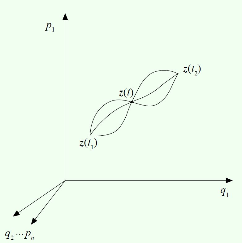
Fig. 1 Phase-space variations of different paths.
Replacing \(L\) by \(L_{ph}\) in \(S = \int L dt\) we define the phase-space action integral
We know from variational calculus that \(S_{ph}\) is stationary under arbitrary variations of the phase-space path (with endpoints fixed), explicitly, we get:
which gives us the Hamilton’s equations:
Note
More generally, the phase-space Lagrangian can depend on \(\dot{p}\) as well, and makes the Lagrange’s equations become:
References
- L.D. Landau & E.M. Lifshitz, Mechanics.
- Lecture notes by Bob Dewar on website Classical Mechanics.