Weyl Semi-metal¶

Graphene¶

In the tight-binding approximation, when only nearest neighborhood couplings are considered, the Hamiltonian of Graphene can be written as:

\[\begin{split}\hat{H}(\vec{k})=-t\begin{pmatrix}0 &h(\vec{k})\\h^*(\vec{k}) &0\end{pmatrix}\end{split}\]

where \(h(\vec{k})=\sum\limits_{\vec{\delta}_i}e^{i\vec{k}\cdot\vec{\delta}_i}=|h(\vec{k})|e^{i\phi(\vec{k})},\vec{\delta}_i\) are three position vectors shown in the following diagram.

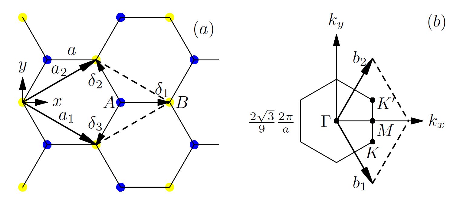
Fig. 1 Crystal Structure of Graphene: \(\vec{a}_{1}\) and \(\vec{a}_{2}\) are Bravais crystal vectors for a Graphene unit cell. Each primitive unit cell has two atomic sties, A and B. \(\vec{\delta}_{i}\) specifies B-s’ position around A site. (b) Brillouin Zone for Graphene \(\vec{b}_{1}\) and \(\vec{b}_{2}\) are reciprocal vector basis for intrinsic Graphene. Its corners are known as K and K’ points.

Then the Hamiltonian is:

\[\begin{split}\hat{H}(\vec{k})=-t|h(\vec{k})|\begin{pmatrix}0 &e^{i\phi(\vec{k})}\\e^{-i\phi(\vec{k})} &0\end{pmatrix}\end{split}\]

with the eigen-value: \(E(\vec{k})=-t|h(\vec{k})|\) and eigen-function (only show one of the two):

\[\begin{split}u(\vec{k})=\frac{1}{\sqrt{2}}\begin{pmatrix}e^{i\phi(\vec{k})/2}\\e^{-i\phi(\vec{k})/2} \end{pmatrix}e^{i\psi(\vec{k})}\end{split}\]

We should notice that the \(1/2\) factor is quite important here, when \(\phi\) changes \(2\pi\), the wave-function does not return to its original value, but with a minus sign. If instead, we want the wave-function to be single valued, the function :math:`psi(vec{k})`should change accordingly.

At the vicinity of Dirac point (K or K’, here we expand the things near K), we have:

\[\begin{split}\hat{H}(\vec{K}+\vec{q})=&\alpha\begin{pmatrix}0&q_x+iq_y\\q_x-iq_y&0\end{pmatrix}=\alpha(q_x\sigma_x-q_y\sigma_y) \\ =&\alpha|q|\begin{pmatrix}0 &e^{i\phi(\vec{q})}\\e^{-i\phi(\vec{q})} &0\end{pmatrix}\end{split}\]

We can see that the general \(\phi\) turn out to be the angle of \(\vec{q}\) with the x axis. Then, wind a circle around the Dirac point K at some energy in the band structure shown below (Fig. 2(a)), the corresponding \(\phi\) (Fig. 2(c))winds one round too.

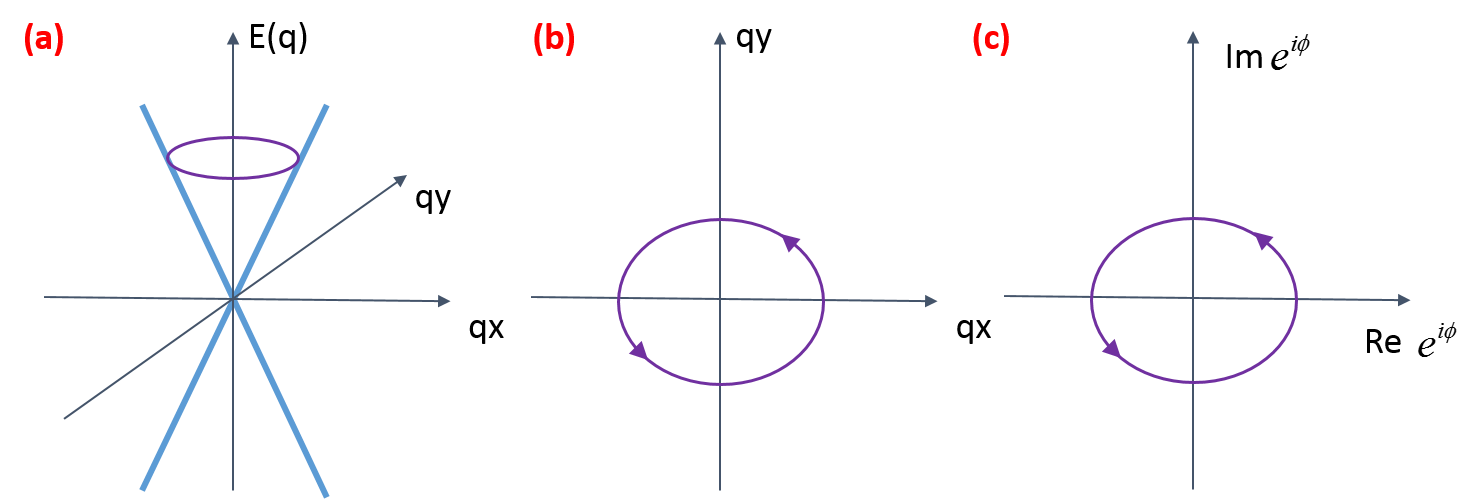
Fig. 2 Dirac cone and the winding of \(\vec{q}\) and \(\phi\)

So, if \(\vec{q}\) circles around the Dirac point one turn, \(\phi\) changes from 0 to \(2\pi\), in order to keep the basic wave-function \(u(\vec{q})\) single-valued, \(\psi\) must changes \(\pi\).

More explicitly, we calculate the vector potential in momentum space with:

\[\vec{A}(\vec{k})=i\langle u^\dagger |\nabla_{\vec{k}} u(\vec{k})\rangle=-\nabla \psi(\vec{k})\]

Then we get:

\[\gamma=\oint{\vec{A}\cdot d\vec{k}} =-\psi(\phi=2\pi)+\psi(\phi(0))=-\pi\]

We got the Berry’s phase \(\gamma=\pm\pi\). It is this non-trivial phase of the equal-frequency surface that makes us call it Weyl semi-metal, and the Dirac points called Weyl nodes.

Three dimension: Weyl semi-metal and Chern number¶

In three dimension, things can goes the same way. Using a simple model with Hamiltonian:

\[H(\vec{k})=\left[-2t_x\left(cosk_x-cosk_0\right)+m\left(2-cosk_y-cosk_z\right)\right]\sigma_x+2t_ysink_y\sigma_y+2t_zsink_z\sigma_z\]

It has two Weyl nodes: \(\vec{K}=\pm\left(k_0,0,0\right)\), which means if we treat \(k_x\) as a variable, only when \(k_x=\pm k_0\), the corresponding energy band \(E_{k_x}(k_y,k_z)\) is crossing at the point \(k_y,k_z=(0,0)\).

Also, at the Weyl node (say \(k_x=k_0\)), we have:

\[H(\vec{K}+\vec{q})=v_xq_x\sigma_x+v_yq_y\sigma_y+v_zq_z\sigma_z\]

with \(v_x=2t_xsink_0,v_y=2t_y,v_z=2t_z\). Without loss of generality, we can set \(v_x=v_y=v_z\) (the only effect is the shape changing from sphere to ellipsoid, which has no effect on the topology), then we get:

\[H(\vec{K}+\vec{q})=v\vec{q}\cdot\vec{\sigma}\]

with eigen-value: \(E(\vec{k})=v|\vec{q}|\) and eigen-function (only show one of the two):

\[\begin{split}u(\vec{k})=\begin{pmatrix}sin\frac{\theta}{2}\\-cos\frac{\theta}{2}e^{i\phi}\end{pmatrix}e^{i\chi}\end{split}\]

It is easy to find that this wave-function will give us a magnetic field with a monopole at \(\vec{K}\), which will give us non-trivial equal-frequency surface Chern number \(C=1\).

Bulk-boundary corresponding¶

In order to see things clearer, also, to see the connection of Weyl semi-metal with Topological insulator, we treat \(k_x\) as a variable, the Hamiltonian is:

\[H_{k_x}(k_y,k_z)=\vec{h}(\vec{k})\cdot\sigma=\left[-2t_x\left(cosk_x-cosk_0\right)+m\left(2-cosk_y-cosk_z\right)\right]\sigma_x+2t_ysink_y\sigma_y+2t_zsink_z\sigma_z\]

For example, we set \(t_x=t_y=t_z=1,m=2,k_0=1\), three typical energy band dispersions shown below:

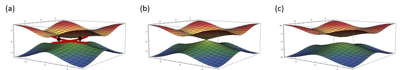
Fig. 3 Typical energy band dispersion with (a) \(k_x=0\), (b) \(k_x=k_0=1\), (c) \(k_x=2\).

To see if the system with \(k_x\neq k_0\) is a topological insulator or not, we can plot the diagram of \(\vec{h}(k_y,k_z)\), and see how many times the resulting torus incorporates the origin point. Typical shape of the torus shows below:

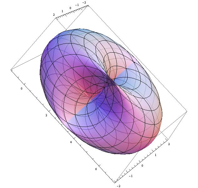
Fig. 4 Typical torus of \(\vec{h}(k_y,k_z)\) with \(k_x=0\).

We found that at the region \(k_x=[-k_0,k_0]\), the origin point is in the torus once with Chern number \(C=1\), outside of that, we got \(C=1\) (Noticing we have \(k_x=[-\pi,\pi]\)) . This is why we plot the edge state in Fig. 4(a), but not in Fig. 4(c). In the non-trivial case, for any energy inside the gap, we get a edge state, so different \(k_x\) will give us a edge-state line, which is called Fermi-arc, especially, when we look at the case of Fermi surface with energy \(E=0\), the Fermi-arc stretch from one Weyl node to another, like the picture shown below:

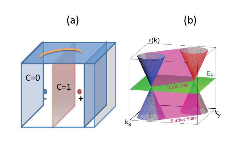
Fig. 5 Fermi arc.

Alternatively, we can look at the Bulk-boundary corresponding another way. The Weyl points behave like “magnetic” monopoles in momentum space whose charge is given by the chirality; they are actually a source of “Berry flux” rather than magnetic flux.

Consider a curve in the surface Brillouin zone encircling the projection of the bulk Weyl point, which is traversed counterclockwise as we vary the parameter \(\lambda: 0 \to 2\pi; \mathbf{k}_{\lambda} = [k_x (\lambda),k_y (\lambda)]\) [see Fig. 6(a)].We show that the energy \(\lambda\) of a surface state at momentum \(\mathbf{k}_{\lambda}\) crosses \(E = 0\) at some value of \(\lambda\). Consider \(H(\lambda,k_z) = H(\mathbf{k}_{\lambda},k_z)\), which can be interpreted as the gapped Hamiltonian of a two-dimensional system (with \(\lambda\) and \(k_z\) as the two momenta). The two periodic parameters \(\lambda\) , \(k_z\) define the surface of a torus in momentum space. The Chern number of this two-dimensional band structure is given by the Berry curvature integration: \(\frac{1}{2\pi}\int\mathscr{F}dk_zd\lambda\), which, by the Stokes theorem, simply corresponds to the net monopole density enclosed within the torus. This is obtained by summing the chiralities of the enclosed Weyl nodes. Consider the case when the net chirality is unity, corresponding to a single enclosed Dirac node. Then, the two-dimensional subsystem is a quantum Hall insulator with unit Chern number. When the system is given a boundary at \(z = 0\), we expect a chiral edge state for this subsystem [see Fig. 6(b)]. Hence, this surface state crosses zero energy somewhere on the surface Brillouin zone \(\mathbf{k}_{\lambda_0}\) . Such a state can be obtained for every curve enclosing the Weyl point. Thus, at zero energy, there is a Fermi line in the surface Brillouin zone, that terminates at the Weyl point momenta [see Fig. 6(c)]. An arc beginning on a Weyl point of chirality c has to terminate on a Weyl point of the opposite chirality. Clearly, the net chirality of the Weyl points within the \((\lambda,k_z)\) torus was a key input in determining the number of these states. If Weyl points of opposite chirality line up along the \(k_z\) direction, then there is a cancellation and no surface states are expected.

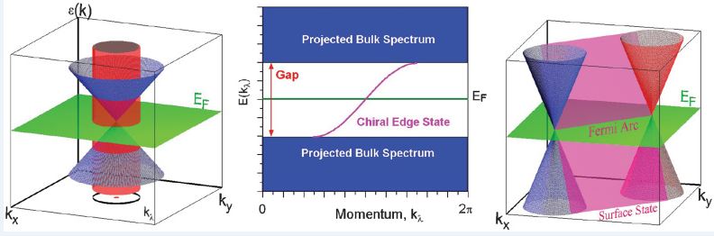
Fig. 6 Illustration of surface states arising from bulk Weyl points.

References:

1. Wan, A.M. Turner, A. Vishwanath, and S.Y. Savrasov, Physical Review B 83, 205101 (2011).
A.M. Turner, A. Vishwanath, and C.O. Head, Topological Insulators 6, 293 (2013).
1. Haldane, Physical Review Letters 93, 206602 (2004).