Lecture 1 : 1-d SSH model¶

The Su-Schrieffer–Heeger (SSH) model¶

The simplest non-trivial topology : 1-d lattice.

Peierls instability makes the atoms dimerize.

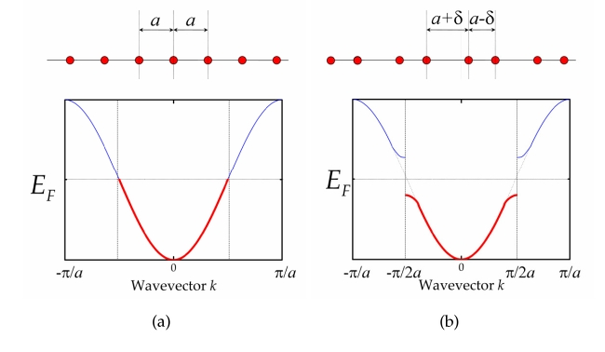
Polyacetylene Structure:

Tight-binding method: first quantization¶

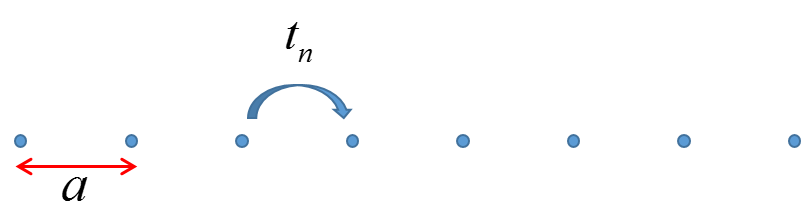
1-d atom chain

Tight-binding method: Single electron total Hamiltonian in atom chain:

\[H=\frac{p^2}{2m}+U(x)\]

with periodical potential: \(U(x+na)=U(x)\)

Assume single atom potential \(V(x)\) with Hamiltonian

\[H_0=\frac{p^2}{2m}+V(x)\]

and well solved eigen-value and eigen-wave-function:(consider only one state)

\[H_0\phi(x)=E_0\phi(x)\]

Do the combination

\[\psi(x)=\sum\limits_n a_n\phi_n\]

with \(\phi_n=\phi(x-x_n), x_n=na\). Define \(\Delta U(x)=U(x)-V(x)\), and substitute following equation

\[H\psi=\left(H_0+\Delta U\right)\psi=E\psi\]

we get

\[\sum_n \langle \phi_m|\Delta U(x-x_n)|\phi_n\rangle a_n=(E-E_0)a_m\]

Define: \(\langle \phi(x-ma+na)|\Delta U(x) |\phi(x)\rangle=-J(x_m-x_n)\)

We get:

\[-\sum_n J(x_m-x_n) a_n=(E-E_0) a_m\]

Because of the Tranformation symmetry of the Hamiltonian, the resulting wavefunction \(\psi(x)\) should take Bloch form, which means we should have the solution \(a_m=e^{ikx_m}\), then, we get

\[E-E_0=-\sum_n J(x_n)e^{-ikx_n}\]

Consider only the nearest-hopping interaction, define \(J_0=J(0), J=J(\pm a)\), then we have:

\[\begin{split}E-E_0+J_0=&-J(e^{ika}+e^{-ika}) \\ =&-2Jcoska\end{split}\]

Second quantization¶

In the second quantization language, the expectation value of energy becomes a operator, set \(\mathscr{H}=\frac{p^2}{2m}+U(x)\), we have

\[H=\langle \psi|\mathscr{H}|\psi \rangle \Rightarrow \hat{H}=\sum_{m,n}\hat{c}_m^\dagger H_{mn}\hat{c}_n\]

with \(\psi \to \hat{\psi}=\sum\limits_n \hat{c}_n \phi_n, H_{mn}=\langle \phi|\mathscr{H}|\phi \rangle\) \(\phi_n\) is a orthonormal and complete basis in Hilbert space, like plane-waves \(e^{ikx}\) or energy eigen-states of \(H_0\), \(\mathscr{H}\) is the energy operator in single particle first quantization picture, which can only act on Hilbert space, while the second quantization energy operator \(\hat{H}\) acts on Fock space. Here, in tight-binding method, \(\phi_n\) is the wave-function of site \(n\) of the energy eigen-state \(H_0\).

Consider only the nearest interaction, we have:

\[\hat{H}=\sum_{n=1}^M \hat{c}_n^\dagger \hat{c}_{n+1}t_n+h.c.\]

\(h.c.\) means hermitian conjugation. Rewrite it in matrix form: \(\hat{H}=\sum\limits_{mn}\hat{c}_m \tilde{H}_{mn}c_n\), we have

\[\begin{split}\tilde{H}_{mn}=\begin{pmatrix} 0 & t_1 &0 & \cdots&t_M^*\\ t_1^* &0&t_2&\cdots&0\\ 0&t_2^*&0&\cdots&0\\ \vdots&\vdots&\vdots&\vdots&\vdots\\ t_M&0&0&t_{M-1}^*&0 \end{pmatrix}\end{split}\]

In the case when \(t=t_n\), \(\hat{c}_n\) satisfy the Bloch condition, we can transform it into momentum space, with \(\hat{c}_n=\frac{1}{\sqrt{M}}\sum\limits_k \hat{c}_k e^{ikx_n}\),

we can easily get

\[\hat{H}=\sum\limits_k \hat{c}_k^\dagger \hat{c}_k(te^{ika}+t^*e^{-ika})=\sum\limits_k \hat{c}_k^\dagger \hat{c}_k E(k)\]

which gives us the dispersion relation:

\[\begin{split}E(k)=&te^{ika}+t^*e^{-ika}\\ =&2tcoska \qquad \textit{for t is real}\end{split}\]

On the other hand, keep in mind that we would get \(c_n=e^{ik(n-1)a}c_1\), that is

\[\begin{split}\hat{H}=\begin{pmatrix}c_1^\dagger&c_2^\dagger&\cdots&c_M^\dagger \end{pmatrix} \begin{pmatrix} 0 & t &0 & \cdots&t^*\\ t^* &0&t&\cdots&0\\ 0&t^*&0&\cdots&0\\ \vdots&\vdots&\vdots&\vdots&\vdots\\ t&0&0&t^*&0 \end{pmatrix} \begin{pmatrix}c_1\\c_2\\\vdots\\c_M\end{pmatrix}\end{split}\]

\[\begin{split}\Rightarrow &\begin{pmatrix}c_1^\dagger&c_1^\dagger e^{-ika}&\cdots&c_1^\dagger e^{-ik(M-1)a} \end{pmatrix} \begin{pmatrix} 0 & t &0 & \cdots&t^*\\ t^* &0&t&\cdots&0\\ 0&t^*&0&\cdots&0\\ \vdots&\vdots&\vdots&\vdots&\vdots\\ t&0&0&t^*&0 \end{pmatrix} \begin{pmatrix}c_1\\c_1 e^{ika}\\\vdots\\c_1e^{ik(M-1)a}\end{pmatrix}\\ =&\begin{pmatrix}c_1^\dagger&\cdots&c_1^\dagger \end{pmatrix} \begin{pmatrix} te^{ika}+t^*e^{-ika} & 0&0\\ 0&\ddots&0\\ 0&0&te^{ika}+t^*e^{-ika} \end{pmatrix} \begin{pmatrix}c_1\\\vdots\\c_1\end{pmatrix}\end{split}\]

which also gives us \(E(k)=te^{ika}+t^*e^{-ika}\).

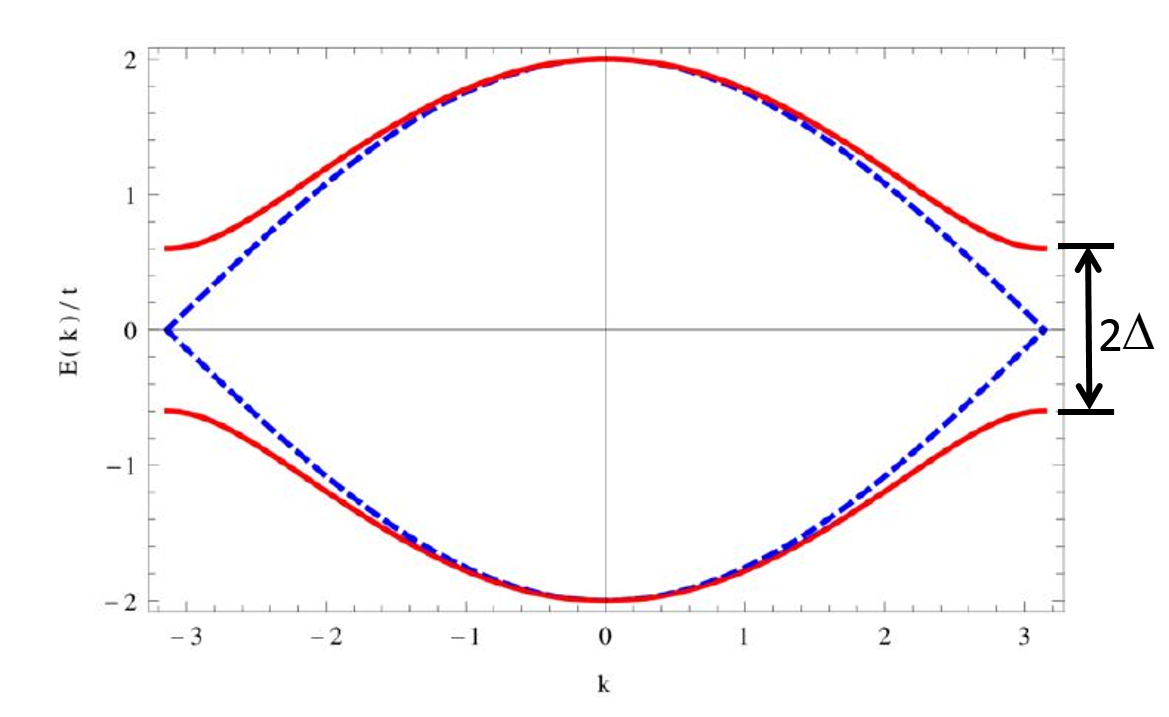
More generally, \(t_n\) can be different from each other, for example, if they are all different up to \(4\), but have a super-periodicity with \(t_{5}=t_1\), then there will have 4 sub-bands, in the example we will consider below, we have two \(t\), \(t_1\neq t_2\), and we have two sub-bands.

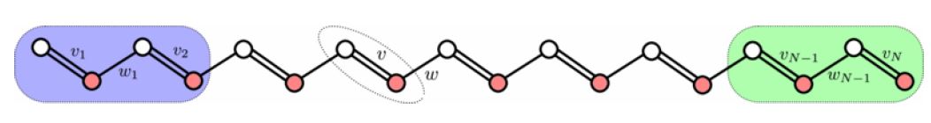
If each atom have a valance electron, then the above mentioned energy band structure \(E(k)=2tcoska\) is not the stable fundamental mode, it will dimerizes to lower the total energy, that means we’ll get following coupling case:

with the Hamiltonian:

\[H=\sum_{n=1}^N(v_n c_{n,1}^\dagger c_{n,2}+w_nc_{n,2}^\dagger c_{n+1,1}+h.c.)\]

with \(M=2N\).

Review¶

In 1-d atom chain, we have got the Hamiltonian in second-quantization frame as:

\[\hat{H}=\sum_{n=1}^M \hat{c}_n^\dagger \hat{c}_{n+1}t_n+h.c.\]

\(h.c.\) means hermitian conjugation. Rewrite it in matrix form: \(\hat{H}=\sum\limits_{mn}\hat{c}_m {H}_{mn}\hat{c}_n\), we have

\[\begin{split}\hat{H}=\begin{pmatrix}c_1^\dagger&c_2^\dagger&\cdots&c_M^\dagger \end{pmatrix}\begin{pmatrix} 0 & t_1 &0 & \cdots&t_M^*\\ t_1^* &0&t_2&\cdots&0\\ 0&t_2^*&0&\cdots&0\\ \vdots&\vdots&\vdots&\vdots&\vdots\\ t_M&0&0&t_{M-1}^*&0 \end{pmatrix}\begin{pmatrix}c_1\\c_2\\\vdots\\c_M\end{pmatrix}\end{split}\]

Energy band and topology¶

\[\begin{split}\hat{H}=\begin{pmatrix}c_1^\dagger&c_2^\dagger&\cdots&c_M^\dagger \end{pmatrix}\begin{pmatrix} 0 & t_1 &0 & \cdots&t_M^*\\ t_1^* &0&t_2&\cdots&0\\ 0&t_2^*&0&\cdots&0\\ \vdots&\vdots&\vdots&\vdots&\vdots\\ t_M&0&0&t_{M-1}^*&0 \end{pmatrix}\begin{pmatrix}c_1\\c_2\\\vdots\\c_M\end{pmatrix}\end{split}\]

\(t_n\) can differ from each other.

For a open chain with \(M\) atoms, we have \(t_M=0\), and this matrix will give us \(M\) eigen-values and eigen-functions.
Possess translational invariance with \(c_{n+1}=c_1e^{ikna}\), it will be diagonalized with \(H(k)=te^{ika}+t^*e^{-ika}\).
Staggered hopping parameters with \(t_1\neq t_2\), but have property \(c_{2n+1}=c_1e^{iknb},c_{2n+2}=c_2e^{iknb}\). We can block the Hamiltonian up in \(2\times 2\) blocks and also pair up \(c_{2n+1},c_{2n+2}\).

The Hamiltonian:

\[H=\sum_{n=1}^N(v_n c_{n,1}^\dagger c_{n,2}+w_nc_{n,2}^\dagger c_{n+1,1}+h.c.)\]

with \(M=2N\).

For a more beautiful notation, define \(\mathbf{c}_n^\dagger=(c_{n,1}^\dagger,c_{n,2}^\dagger)=(c_{2n-1}^\dagger,c_{2n}^\dagger)\), then we have

\[H=\sum_{m,n=1}^N \mathbf{c}_m^\dagger H_{mn}\mathbf{c}_n\]

with

\[\begin{split}\mathbf{c}_n^\dagger H_{nn}\mathbf{c}_n=\begin{pmatrix}c_{n,1}^\dagger&c_{n,2}^\dagger\end{pmatrix}\begin{pmatrix}0&v_n\\v_n^*&0\end{pmatrix}\begin{pmatrix}c_{n,1}\\c_{n,2}\end{pmatrix}=\begin{pmatrix}c_{n,1}^\dagger&c_{n,2}^\dagger\end{pmatrix}U_n\begin{pmatrix}c_{n,1}\\c_{n,2}\end{pmatrix}\end{split}\]

and

\[\begin{split}\mathbf{c}_n^\dagger H_{nn+1}\mathbf{c}_{n+1}=\begin{pmatrix}c_{n,1}^\dagger&c_{n,2}^\dagger\end{pmatrix}\begin{pmatrix}0&0\\w_n&0\end{pmatrix}\begin{pmatrix}c_{n+1,1}\\c_{n+1,2}\end{pmatrix}=\begin{pmatrix}c_{n,1}^\dagger&c_{n,2}^\dagger\end{pmatrix}T_n\begin{pmatrix}c_{n+1,1}\\c_{n+1,2}\end{pmatrix}\end{split}\]

\[\begin{split}\mathbf{c}_{n+1}^\dagger H_{n+1n}\mathbf{c}_{n}=\begin{pmatrix}c_{n+1,1}^\dagger&c_{n+1,2}^\dagger\end{pmatrix}T_n^\dagger\begin{pmatrix}c_{n,1}\\c_{n,2}\end{pmatrix}\end{split}\]

when \(|m-n|>1\), we have \(H_{mn}=0\).

For example, for 6 cells (12 sites), we have

\[\begin{split}H=\begin{pmatrix}U_1&T_1&0&\cdots&T_6^\dagger\\ T_1^\dagger&U_2&T_2&\cdots&0\\ 0&T_2^\dagger&U_3&\cdots&0\\ \vdots&\vdots&\vdots&\vdots&\vdots\\ T_6&0&0&\cdots&U_6 \end{pmatrix}\end{split}\]

\[\begin{split}H_{mn}=\begin{pmatrix}U_1&T_1&0&\cdots&T_6^\dagger\\ T_1^\dagger&U_2&T_2&\cdots&0\\ 0&T_2^\dagger&U_3&\cdots&0\\ \vdots&\vdots&\vdots&\vdots&\vdots\\ T_6&0&0&\cdots&U_6 \end{pmatrix}\end{split}\]

Open chain: \(T_6=0\).
Closed chain with translational symmetry, \(T_n=T,U_n=U\), with

\[\begin{split}U=\begin{pmatrix}0&v\\v^*&0\end{pmatrix},T=\begin{pmatrix}0&0\\w&0\end{pmatrix}\end{split}\]

Using three Pauli matrices

\[\begin{split}\sigma_x=\begin{pmatrix}0&1\\1&0\end{pmatrix},\sigma_y=\begin{pmatrix}0&-i\\i&0\end{pmatrix},\sigma_z=\begin{pmatrix}1&0\\0&-1\end{pmatrix}\end{split}\]

We get

\[U=Re(v)\sigma_x-Im(v)\sigma_y,T=\frac{1}{2}w(\sigma_x-i\sigma_y)\]

Using \(\mathbf{c}_n=e^{ik(n-1)b}\mathbf{c}_1\), we have

\[\begin{split}\hat{H}=\begin{pmatrix}\mathbf{c}_1^\dagger&\mathbf{c}_2^\dagger&\cdots&\mathbf{c}_N^\dagger \end{pmatrix} \begin{pmatrix} U & T &0 & \cdots&T^\dagger\\ T^\dagger &U&T&\cdots&0\\ 0&T^\dagger&U&\cdots&0\\ \vdots&\vdots&\vdots&\vdots&\vdots\\ T&0&0&T^\dagger&U \end{pmatrix} \begin{pmatrix}\mathbf{c}_1\\\mathbf{c}_2\\\vdots\\\mathbf{c}_N\end{pmatrix}\end{split}\]

\[\begin{split}\Rightarrow \begin{pmatrix}\mathbf{c}_1^\dagger&\mathbf{c}_1^\dagger e^{-ikb}&\cdots&\mathbf{c}_1^\dagger e^{-ik(N-1)b} \end{pmatrix} \begin{pmatrix} U & T &0 & \cdots&T^\dagger\\ T^\dagger &U&T&\cdots&0\\ 0&T^\dagger&U&\cdots&0\\ \vdots&\vdots&\vdots&\vdots&\vdots\\ T&0&0&T^\dagger&U \end{pmatrix} \begin{pmatrix}\mathbf{c}_1\\\mathbf{c}_1 e^{ikb}\\\vdots\\\mathbf{c}_1e^{ik(N-1)b}\end{pmatrix}\end{split}\]

\[\begin{split}=\begin{pmatrix}\mathbf{c}_1^\dagger&\cdots&\mathbf{c}_1^\dagger \end{pmatrix} \begin{pmatrix} U+Te^{ikb}+T^\dagger e^{-ikb} & &\\ &\ddots&\\ &&U+Te^{ikb}+T^\dagger e^{-ikb} \end{pmatrix} \begin{pmatrix}\mathbf{c}_1\\\vdots\\\mathbf{c}_1\end{pmatrix}\end{split}\]

which gives us \(H=H(k)\oplus H(k)\cdots \oplus H(k)=\oplus_{n=1}^N H(k)\) with

\[H(k)=U+Te^{ikb}+T^\dagger e^{-ikb}=\mathbf{h}(k)\cdot \mathbf{\sigma}\]

with

\[\begin{split}h_x(k)=&Re(v)+|w|cos(kb+arg(w))\\ h_y(k)=&-Im(v)+|w|sin(kb+arg(w))\\ h_z(k)=&0\end{split}\]

with \(w=|w|e^{i arg(w)}\).

\[H(k)=\mathbf{h}(k)\cdot \mathbf{\sigma}\]

with

with eigen-energy

\[E(k)=|\mathbf(h)(k)=\pm \sqrt{h_x^2+h_y^2+h_z^2}=\pm \sqrt{|v|^2+|w|^2+2|v||w|cos(kb+arg(v)+arg(w))}\]

and eigen-wavefunctions

\[\begin{split}|\pm\rangle=\begin{pmatrix}\pm e^{-i\phi(k)}\\ 1\end{pmatrix}\end{split}\]

with \(tan\phi=h_y/h_x\).

For example, set \(arg(v)=arg(w)=0\), we have

Can not tell the difference \(|v|-|w|=\pm\delta\).

Energy-band description is not completed, it can give us many information, but not the whole, others are hidden in the wave-function. Alternatively, recalling \(H(k)=\mathbf{h}(k)\cdot \mathbf{\sigma}\), the Hamiltonian should contain the whole information, but we have only used \(|h|\), in topological aspect, \(\mathbf{h}(k)\) will suffices.

Set \(arg(v)=0\),\(kb=[0,2\pi]\), we have two cases

\(|w|<|v|, \mathbf{inter}<\mathbf{intra}\)
\(|w|>|v|, \mathbf{inter}>\mathbf{intra}\)

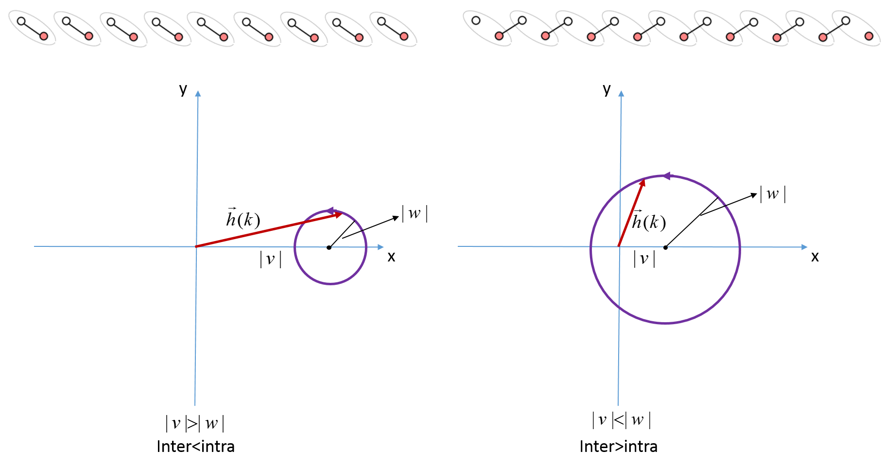
two cases

Winding number¶

\(H(k)=\mathbf{h}(k)\cdot \mathbf{\sigma}\), \(\mathbf{h}(k)=0\) is a degenerate point with \(|v|=|w|\), two bands cross, define \(h(k)=h_x(k)+ih_y(k)\), we have

\[\begin{split}H(k)=\begin{pmatrix}0&h^*(k)\\h(k)&0\end{pmatrix}\end{split}\]

\[ln(h)=ln(|h|)e^{iarg(h)}=ln(|h|)+iarg(h)\]

define

\[\nu=\frac{1}{2\pi i}\int_{-\pi}^{\pi}dk\frac{d}{dk}ln(h(k))\]

When

\(|w|>|v|, \nu=1, \mathbf{inter}>\mathbf{intra}\)
\(|w|<|v|, \nu=0, \mathbf{inter}<\mathbf{intra}\)

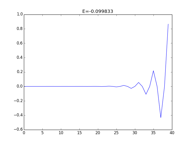
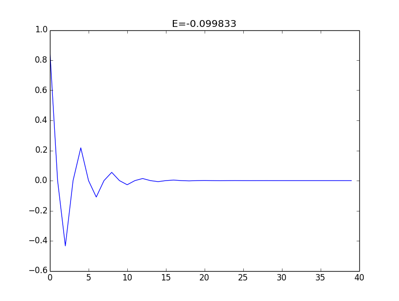
A example, \(N=20, M=2N=40, w=1, v=0.5\), we get eigen-energys:

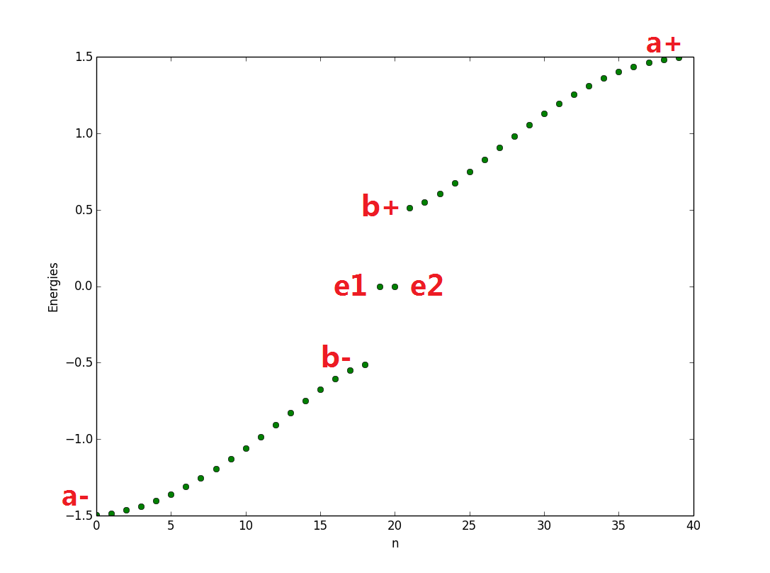
eigen-energy

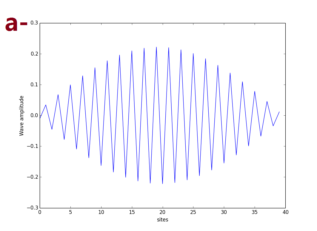
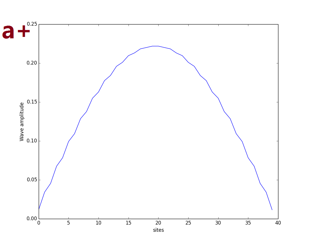
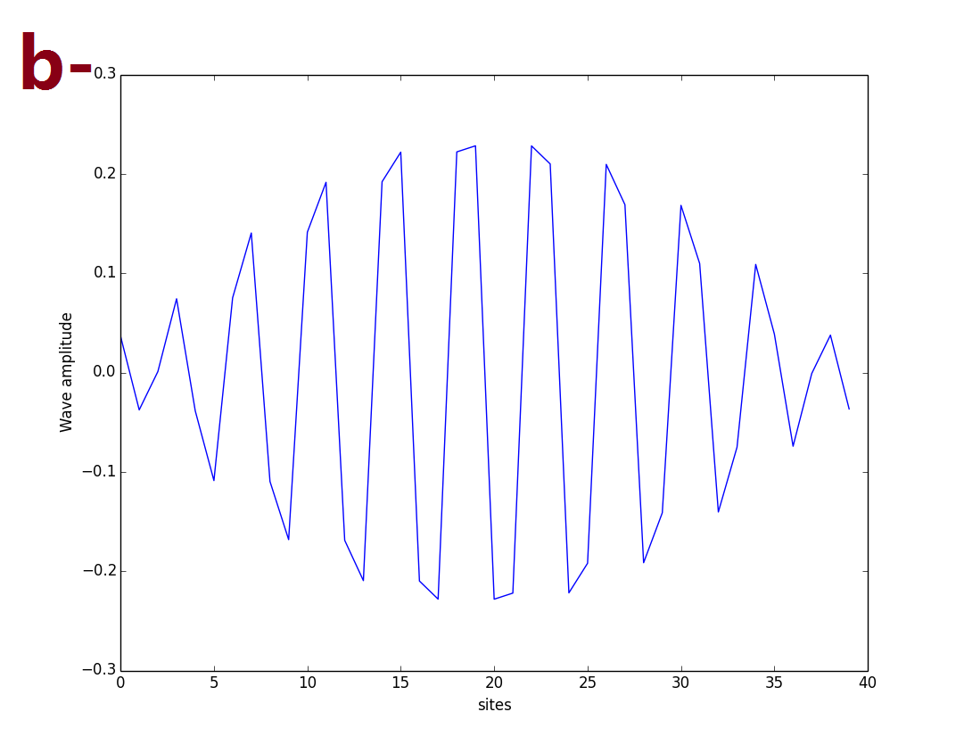
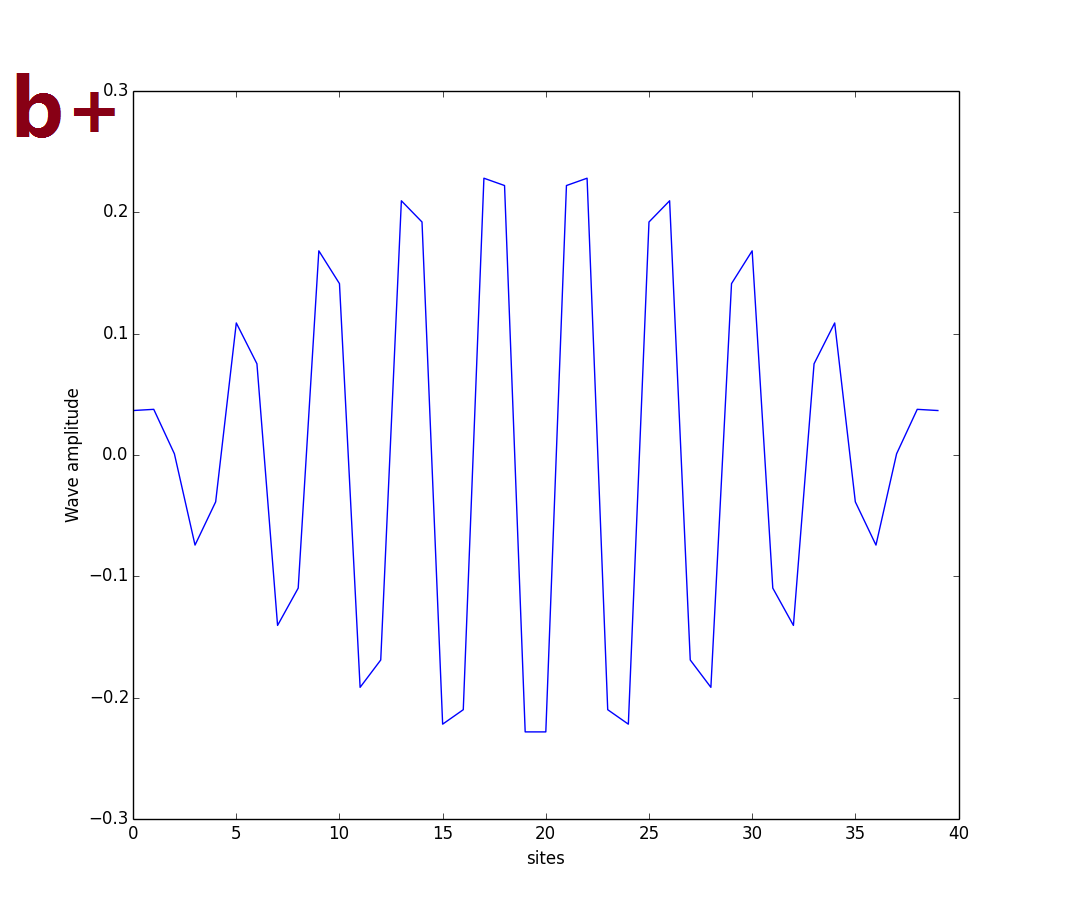
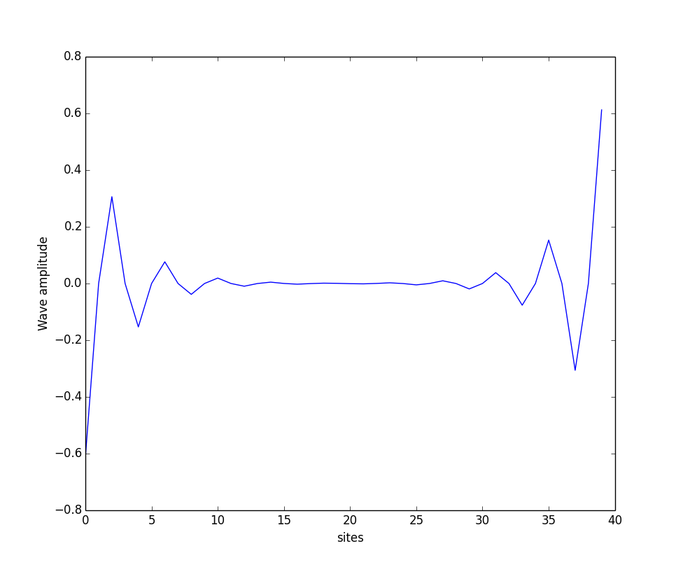
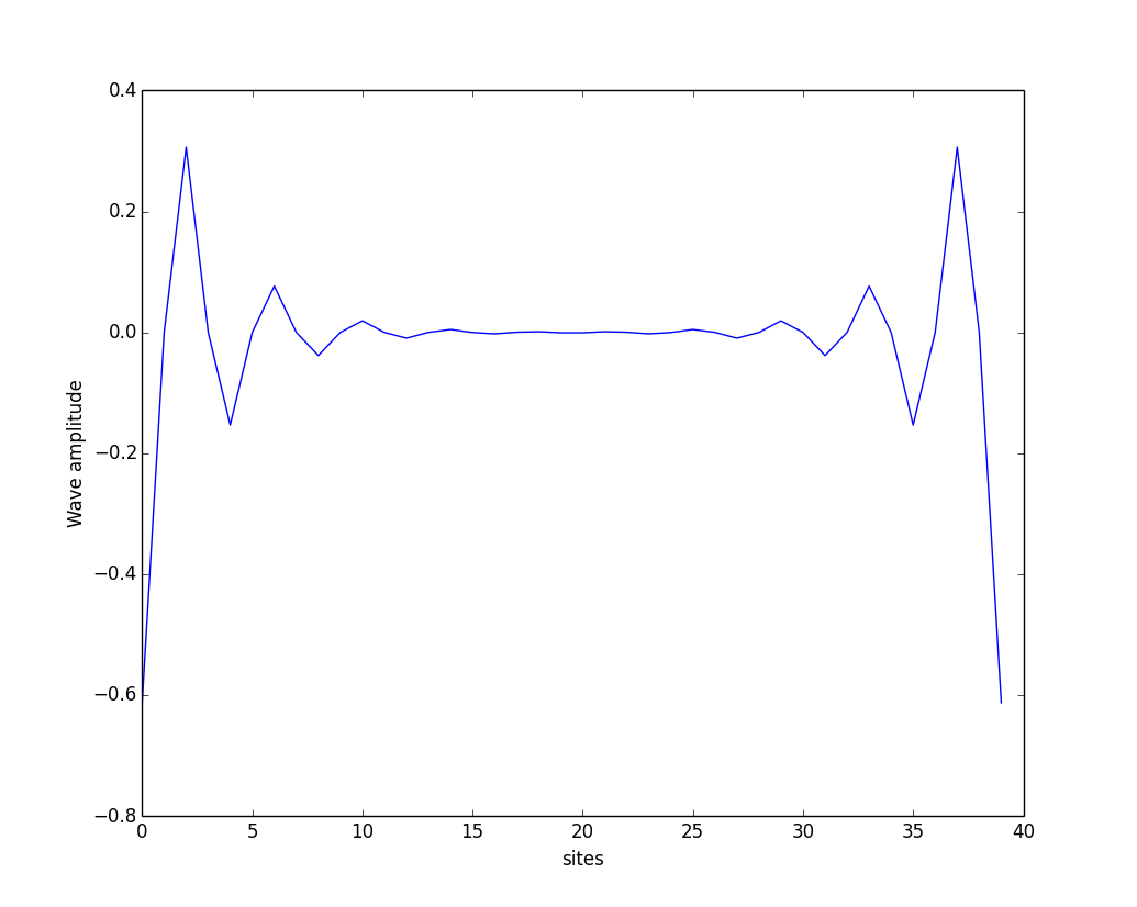
Edge-states:

Chiral symmetry¶

Recalling the Hamiltonian:

\[H=\sum_{n=1}^N(v_n c_{n,1}^\dagger c_{n,2}+w_nc_{n,2}^\dagger c_{n+1,1}+h.c.)\]

Define projector operators:

\[P_A=\sum_n c_{n,1}^\dagger c_{n,1}, P_B=\sum_n c_{n,2}^\dagger c_{n,2}\]

and the chiral operator \(\Sigma_z=P_A-P_B\), The matrix elements of \(\Sigma_z\) vanish, \(\langle 0|c_r \Sigma c^\dagger_s|0\rangle=0\) if sites \(r\) and \(s\) are in different unit cells.

In first-quantization, we have

\[H=\sum_{n=1}^N(v_n |n,1\rangle\langle n,2|+w_n|n,2\rangle\langle n+1,1|+h.c.)\]

and

\[P_A=\sum_n |n,1\rangle\langle n,1|, P_B=\sum_n |n,2\rangle\langle n,2|\]

In matrix form, we have

\[\Sigma_z=\sigma_z\oplus\sigma_z\oplus\cdots\oplus\sigma=\oplus_{n=1}^N \sigma_z\]

\(\Sigma_z\) is local, it does not mix site between unit cells, and inherits the algebra from \(\sigma_z\):

\[\Sigma_z^\dagger\Sigma_z=1\]

\[\Sigma_z^2=1\]

Recalling

\[\begin{split}\begin{pmatrix} U_1 & T_1 &0 & \cdots&T_N^\dagger\\ T_1^\dagger &U_2&T_2&\cdots&0\\ 0&T_2^\dagger&U_3&\cdots&0\\ \vdots&\vdots&\vdots&\vdots&\vdots\\ T_N&0&0&T_{N-1}^\dagger&U_N \end{pmatrix}\end{split}\]

There are no onsite terms in the Hamiltonian, so we have

\[\Sigma_z H \Sigma_z=-H\]

This is the chiral symmetry.

Note

Actually, here, \(H\) is defined in momentum space, but \(\Sigma_z\) in real space, we should write \(\tilde{H}=U^\dagger H U\) for some unitary matrix \(U\), but the property survives!

Consequences: For eigenstates \(|\psi_n\rangle\) of \(H\), we have

\[H|\psi_n\rangle=E_n|\psi_n\rangle\]

\[H\Sigma_z|\psi_n\rangle=-\Sigma_zH|\psi_n\rangle=-\Sigma_zE_n|\psi_n\rangle=-E_n\Sigma_z|\psi_n\rangle\]\[If\]

\(E_n\neq 0\), two orthonormal states \(|\psi_n\rangle, \Sigma_z|\psi_n\rangle\), which gives

\[\begin{split}\begin{pmatrix}\alpha^* &\beta^*\end{pmatrix}\begin{pmatrix}\alpha\\-\beta\end{pmatrix}=0\end{split}\]

\[\Rightarrow |\alpha|^2=|\beta|^2\]
\(E_n=0\), we particularly have \(\Sigma_z=\Sigma_zH\), \(|\psi_n\rangle\) can be eigen-states of \(H\) and \(\Sigma\) simultaneously, \(\Sigma_z|\psi_n\rangle=\pm|\psi_n\rangle\), gives \(|\psi_n\rangle=\begin{pmatrix}1 \\0\end{pmatrix}\) or \(|\psi_n\rangle=\begin{pmatrix}0 \\1\end{pmatrix}\)

Review 2¶

In the last class, we have solved 1-d atom chain with staggered hopping parameters and got the Hamiltonian:

\[\begin{split}H(k)=\mathbf{h}(k)\cdot \mathbf{\sigma}=\begin{pmatrix}0&h_x-ih_y\\h_x+ih_y&0\end{pmatrix}=|h(k)|\begin{pmatrix}0&e^{-i\phi(k)}\\e^{i\phi(k)}&0\end{pmatrix}\end{split}\]

with \(tan\phi=h_y/h_x\).

Eigen-values are \(E(k)=\pm|h(k)|\), with eigen-functions: \(|\pm\rangle=\begin{pmatrix}\pm e^{-i\phi(k)}\\ 1\end{pmatrix}\).

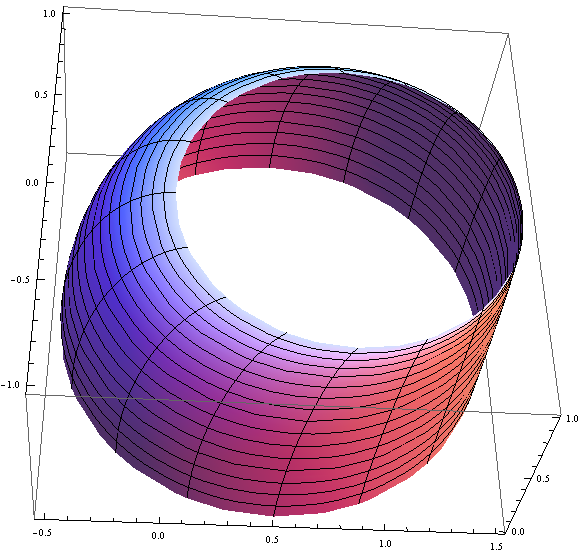
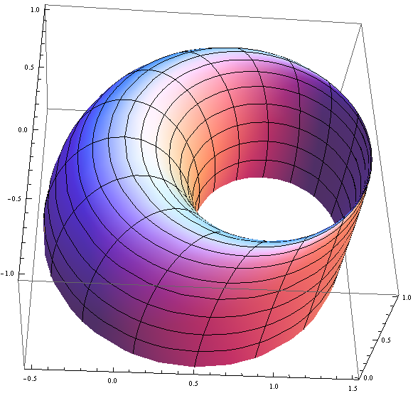
\(\mathbf{h}(k)\) depicted as follow:

Topological transition

Topological transition¶

We have already seen, for \(|w|>|v|\) or \(|w|<|v|\), we got different winding number, means there is a topological transition at \(|w|=|v|\). In the energy-band point of view, it means the gap between two energy bands closes (across each other) and reopens. There are two ways to change the winding number and get a topological transition:

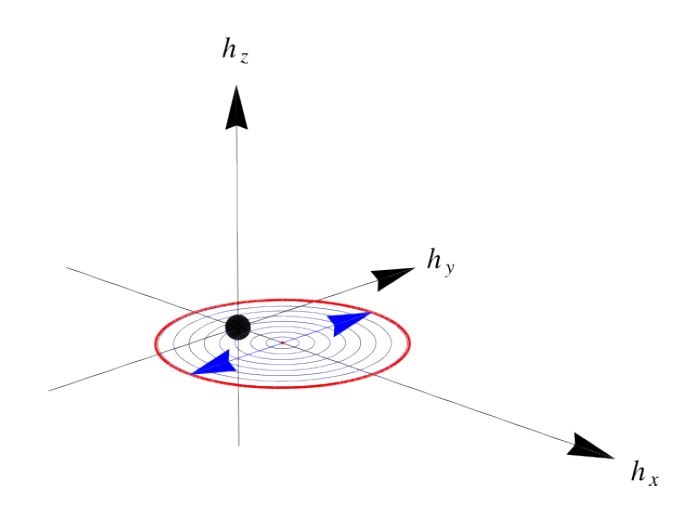
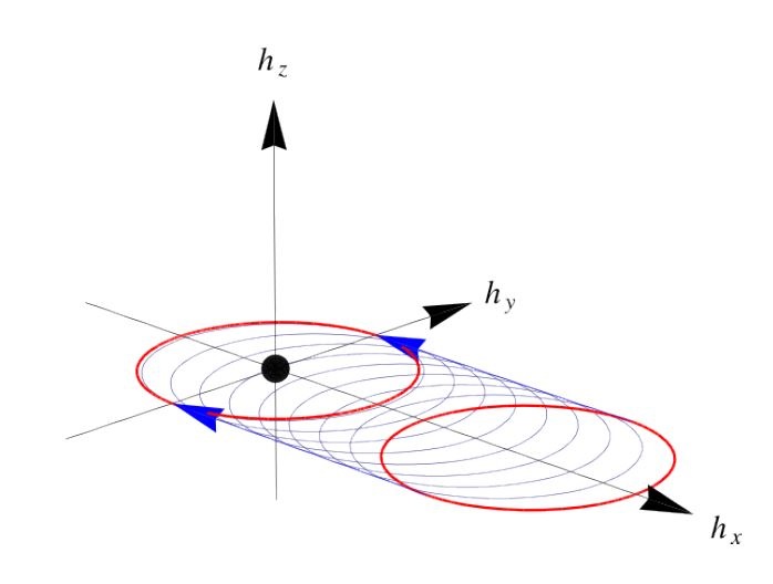
Pull the path through the origin in the \(h_x-h_y\) plane.
Lift it out of the plane (breaking the chiral symmetry).

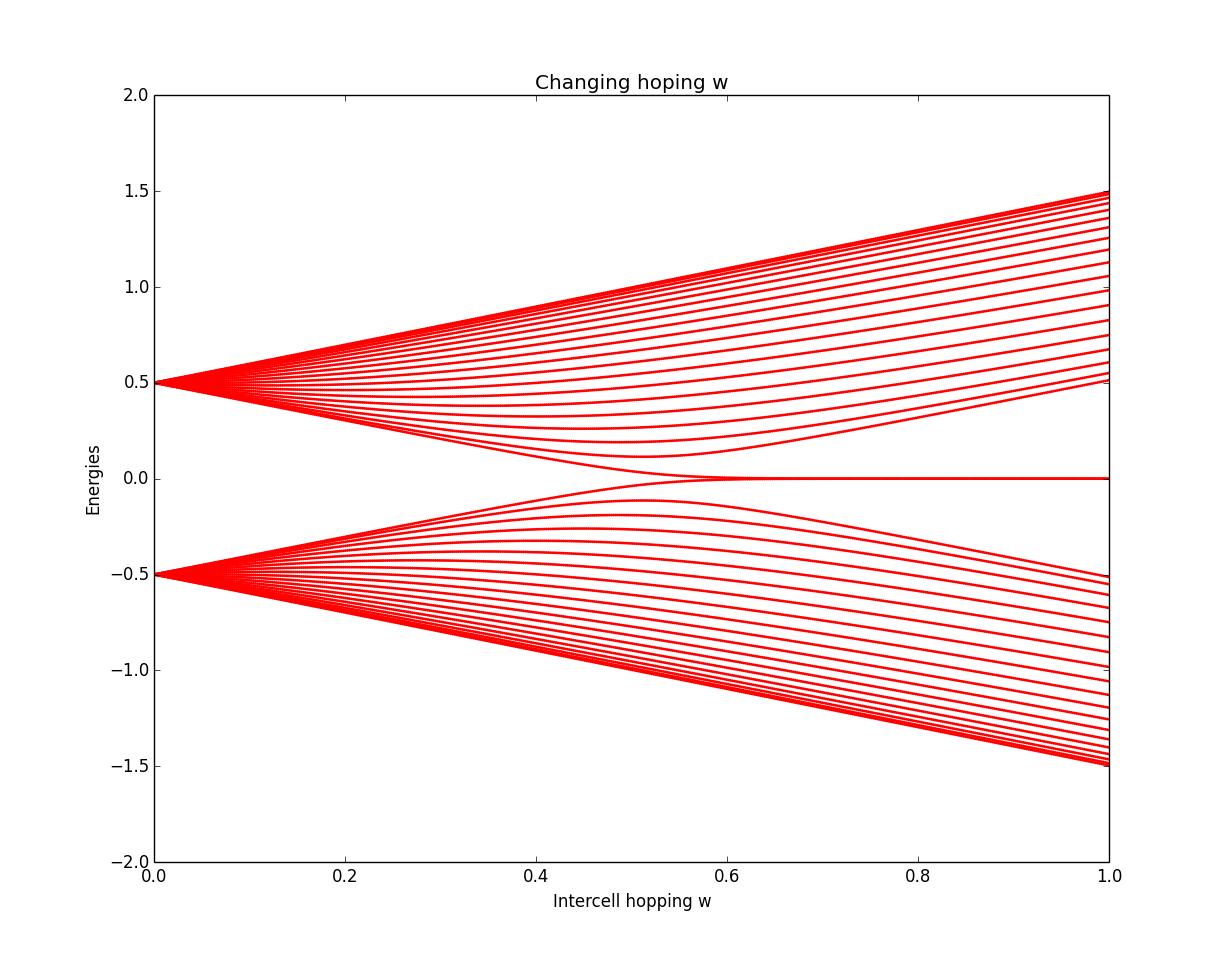
Case 1(a): \(v=0.5, w=0\to 1\)

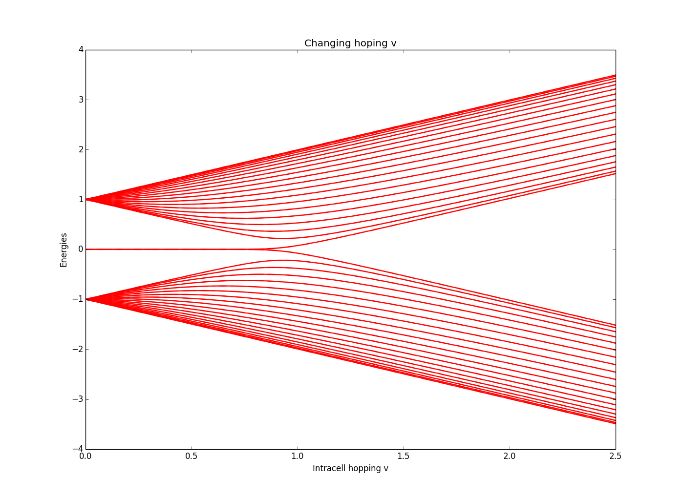
Case 1(b): \(w=1, v=2.5\to 0\)

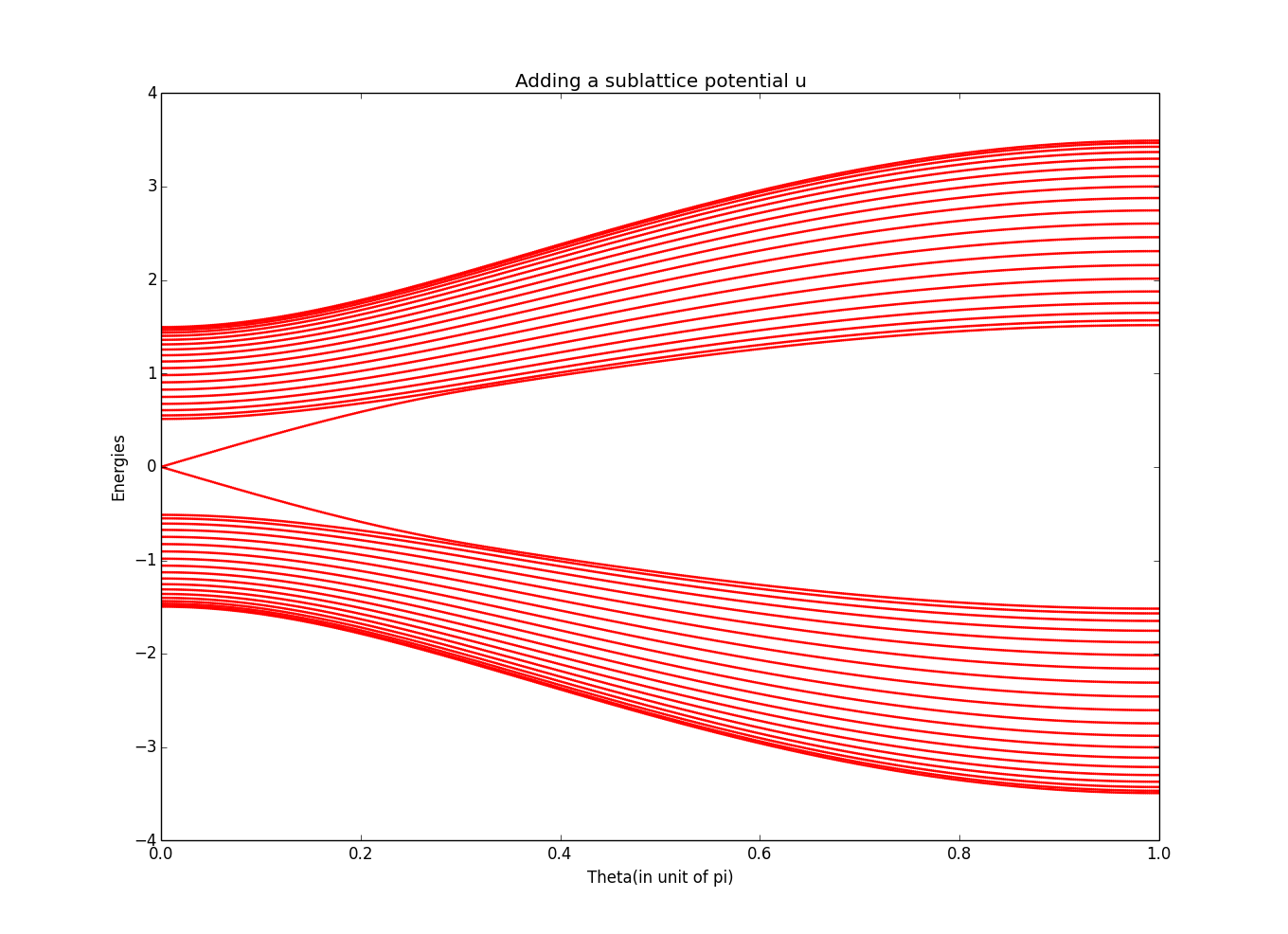
Case 2: Sublattice potential \(H_{sublattice}=u\sigma_z\). Recalling

\[H(k)=U+Te^{ikb}+T^\dagger e^{-ikb}\]

with \(U=\begin{pmatrix}0&v\\v^*&0\end{pmatrix},U=\begin{pmatrix}0&0\\w&0\end{pmatrix}\), now \(U\) changes to \(U=\begin{pmatrix}u&v\\v^*&-u\end{pmatrix}\), and \(H(k)=\mathbf{h}(k)\cdot\mathbf{\sigma}\) with \(h_z(k)=u\).

Set \(w=1, v=1.5-cos\theta, u=sin\theta, \theta=0\to \pi\),

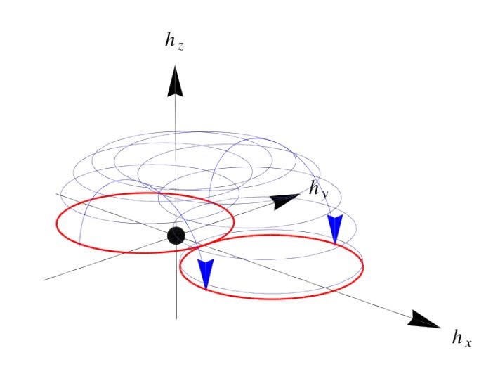
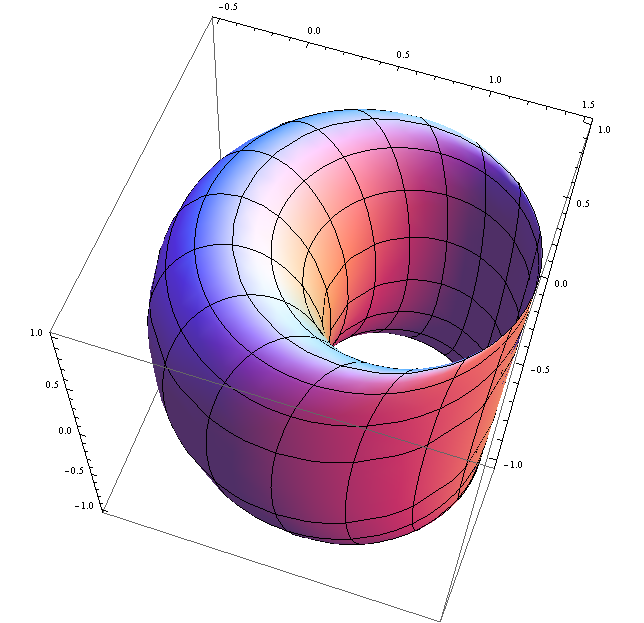
Case 3: Charge Pump: Using the Hamiltonian \(H=u(t)\sum\limits_{i=1}^N(-1)^{i-1}c_i^{\dagger}c_i+\sum\limits_{i=1}^N[t_0+\delta(t)(-1)^i](c_i^{\dagger}c_{i+1}+h.c.)\), with \(u(t)=u_0 sin\theta, \delta(t)=\delta_0 cos\theta\), add time variation with \(\theta=2\pi t/T\), in previous notation, \(v=t_0-\delta(t), w=t_0+\delta(t)\). set \(u=sin\theta, v=0.75-0.25cos\theta, w=0.75+0.25cos\theta\), the vector \(\vec{h(k)}\) is

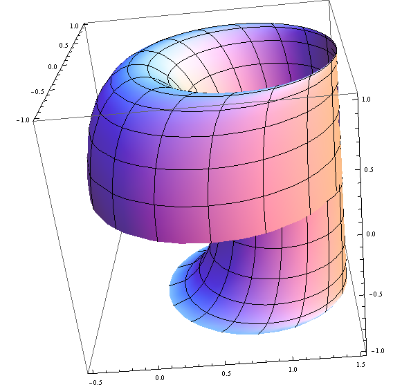
The energy band evolution is

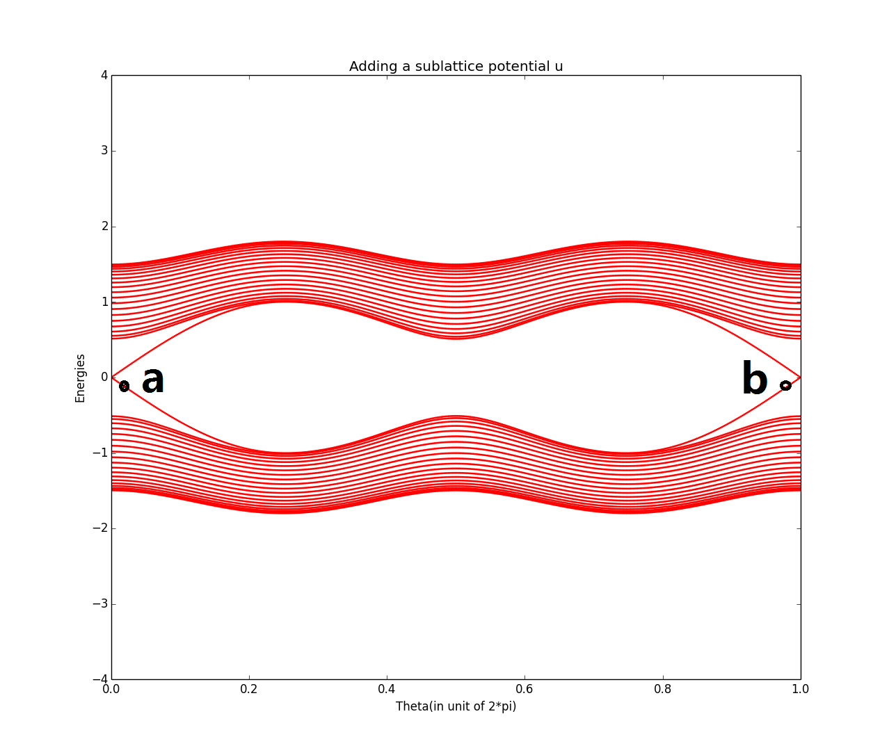
energy4

Winding number v.s. Zak phase¶

From

\[\begin{split}H(k)=\begin{pmatrix}0&h^*(k)\\h(k)&0\end{pmatrix}\end{split}\]

\[ln(h)=ln(|h|)e^{iarg(h)}=ln(|h|)+iarg(h)\]

We have defined the winding number

\[\nu=\frac{1}{2\pi i}\int_{-\pi}^{\pi}dk\frac{d}{dk}ln(h(k))=\frac{1}{2\pi}arg(h)\left.\right|_{-\pi}^{\pi}=1 \ \textit{or}\ 0\]

From the Zak phase definition:

\[\gamma=i\oint\langle\psi|\nabla_k|\psi\rangle\]

Recalling \(|\psi\rangle=\frac{1}{\sqrt{2}}\begin{pmatrix}\pm e^{-i\phi(k)}\\ 1\end{pmatrix}\Rightarrow\gamma=\frac{1}{{2}}\oint dk\nabla_k\phi=\pm\pi \ \textit{or}\ 0\).